
Why Bond Pricing Matters Beyond Finance
When you discount a stream of future cash flows to determine what an asset is worth today, you make an implicit assumption about interest rates. In many introductory treatments, that assumption is brutally simple: a single, flat discount rate applied uniformly across all maturities. If you’ve built pricing models under this assumption, you’ve already encountered its limitations. Real-world interest rates are not flat. A 2-year government bond and a 10-year government bond almost never offer the same annualized yield. The relationship between interest rates and their corresponding maturities—the term structure of interest rates—is one of the most fundamental constructs in fixed-income pricing, and understanding it unlocks a deeper layer of quantitative reasoning.
Why This Matters for Quantitative Practitioners
For data scientists and ML engineers, bond pricing might seem like a narrow domain concern. It isn’t. The term structure underpins:
- Discounted cash flow (DCF) models used across corporate finance, real estate, and startup valuation
- Risk-neutral pricing frameworks central to derivatives modeling
- Macroeconomic signal extraction—yield curve inversions, for instance, are among the most studied recession predictors
- Portfolio optimization and duration/convexity hedging in any fixed-income or multi-asset strategy
The standard progression in quantitative finance curricula makes this explicit: introductory lessons price fixed-income instruments by discounting all future cash flows using a single interest rate, such as the yield-to-maturity. The term structure framework relaxes this assumption by acknowledging that interest rates vary with time-to-maturity. That single conceptual shift—from one rate to a curve of rates—changes everything about how you model, hedge, and interpret fixed-income securities.
The Core Building Blocks
At its heart, the term structure gives rise to three interrelated rate concepts you need to internalize:
- Spot rates: the yield on a zero-coupon instrument from today to a specific future date. Each maturity has its own spot rate.
- Forward rates: the implied future interest rate between two future dates, contracted today. For example, the one-year forward rate represents the return between year 1 and year 2, locked in at time zero.
- Discount factors: derived directly from spot rates, where maps each future cash flow back to its present value.
These aren’t independent quantities. Forward rates are algebraically determined by spot rates, and spot rates are constructed from observable market prices. The expectations hypothesis ties them together economically, positing that forward rates reflect the market’s expectation of future spot rates.
In the sections that follow, we’ll build each of these concepts from first principles, derive their mathematical relationships, and implement them in code—giving you both the theoretical grounding and the practical toolkit to work with real yield curve data.
What Is the Term Structure of Interest Rates?
In fixed-income pricing, a common simplification is to discount all future cash flows using a single interest rate—typically the yield-to-maturity (YTM) or a market reference rate plus a spread. While convenient, this approach ignores a fundamental reality: interest rates vary with time-to-maturity. The term structure of interest rates captures exactly this relationship, mapping yields to their corresponding maturities at a single point in time.
The Core Idea
The term structure answers a straightforward question: what annualized rate of return does the market demand for locking up capital over different horizons? A 2-year bond and a 10-year bond generally don’t offer the same yield. The term structure formalizes this observation into a curve—often called the yield curve—that serves as the foundation for pricing any fixed-income instrument.
For those with a quantitative background, think of the term structure as a function that maps each maturity to a corresponding interest rate. This function is not directly observable for all maturities; it must be estimated or bootstrapped from market data, typically using prices of government bonds or interest rate swaps that are considered default-free.
Why It Matters
The term structure is not merely descriptive—it is the pricing engine for fixed-income markets. Once you have it, you can:
- Price any bond by discounting each cash flow at the maturity-appropriate rate rather than a single flat rate
- Derive forward rates that encode the market’s expectations (or required compensation) for future borrowing costs
- Compute discount factors that translate future cash flows into present values
- Identify relative value—determine whether a bond is cheap or rich relative to the curve
Shapes and Signals
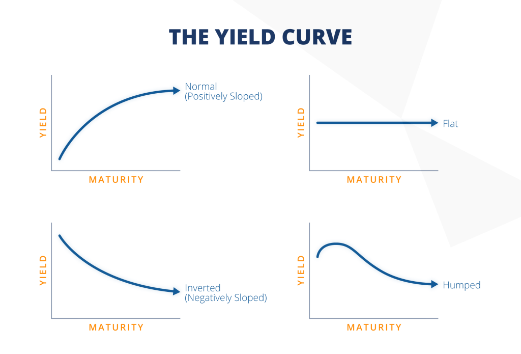
The term structure typically takes one of three shapes, each carrying distinct economic implications:
- Normal (upward-sloping): Long-term rates exceed short-term rates, reflecting compensation for duration risk or expectations of rising rates.
- Inverted (downward-sloping): Short-term rates exceed long-term rates, historically associated with impending economic slowdowns.
- Flat: Rates are roughly uniform across maturities, often signaling a transition between the other two regimes.
From Theory to Practice
The ideal data for constructing the term structure comes from default-free, zero-coupon instruments—securities that make a single payment at maturity. In practice, such instruments exist only for limited maturities (e.g., Treasury bills up to one year), so analysts bootstrap or fit models to coupon-bearing bond prices to extract the underlying term structure. This bootstrapping process produces spot rates, which we explore in the next section.
Spot Rates: The Building Blocks of Bond Pricing
With the term structure established as our conceptual framework, we now turn to its most fundamental output: spot rates. These are the discount rates used to price individual cash flows occurring at specific future dates. Unlike yield-to-maturity, which applies a single rate across all maturities, spot rates respect the core insight of term structure analysis: interest rates vary with time-to-maturity.
What Exactly Is a Spot Rate?
A spot rate is the annualized return on a zero-coupon bond that matures at time , contracted today. It tells you the market’s required rate of return for locking up capital from now until a specific future date. Each maturity has its own spot rate, and collectively, these rates form the spot rate curve (also called the zero-coupon yield curve).
The discount factor for a cash flow occurring at time follows directly:
This discount factor converts a future dollar into its present value equivalent.
From Single-Rate Discounting to the Spot Curve
Traditional bond pricing discounts all future cash flows using a single interest rate. The spot rate approach assigns a unique rate to each cash flow based on its timing. For a coupon bond paying cash flows , the price becomes:
Each cash flow gets its own discount rate. This produces more accurate pricing, especially when the yield curve is steep or non-linear.
Why Spot Rates Matter for Quantitative Work
For data scientists and ML engineers working in fixed-income analytics, spot rates serve as the atomic inputs to pricing models. They enable:
- Arbitrage-free pricing: Consistent valuation across instruments with different maturities
- Curve construction: Bootstrapping spot rates from observable market prices
- Risk decomposition: Measuring sensitivity to rate changes at specific tenors (key rate durations)
The ideal source data comes from liquid government securities or interest rate swaps, where credit risk is minimal and the pure time-value-of-money component can be isolated.
Extracting Spot Rates in Practice
Since zero-coupon bonds don’t exist at every maturity, practitioners bootstrap spot rates from coupon-bearing instruments. The process iteratively solves for each successive spot rate using previously determined rates—a technique that maps naturally to algorithmic implementation and which we’ll walk through in detail in the bootstrapping section below.
With spot rates in hand, we can now derive the rates that describe what happens between future dates—forward rates.
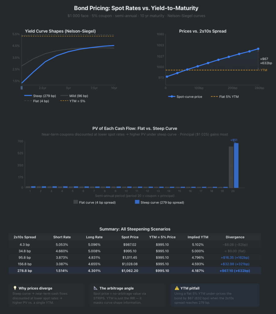
Python Code for Bond Pricing Using Spot Rates vs. a Single YTM
"""
Bond Pricing: Spot Rates vs. Yield-to-Maturity
================================================
Demonstrates two equivalent approaches to pricing a coupon bond:
  1. Discounting each cash flow by its period-specific spot rate
  2. Discounting all cash flows by a single flat yield-to-maturity (YTM)
"""

# ── Bond parameters
FACE_VALUE   = 1_000       # Par value ($)
COUPON_RATE  = 0.05        # Annual coupon rate (5%)
FREQUENCY    = 2           # Semi-annual payments
MATURITY     = 5           # Years to maturity
PERIODS      = MATURITY * FREQUENCY          # Total coupon periods
COUPON       = FACE_VALUE * COUPON_RATE / FREQUENCY   # Per-period coupon ($)

# ── Spot rate curve (bootstrapped / observed), one per semi-annual period
# Format: {period: annualised spot rate}
SPOT_RATES = {
    1:  0.030,   # 0.5 yr
    2:  0.032,   # 1.0 yr
    3:  0.034,   # 1.5 yr
    4:  0.036,   # 2.0 yr
    5:  0.038,   # 2.5 yr
    6:  0.040,   # 3.0 yr
    7:  0.042,   # 3.5 yr
    8:  0.044,   # 4.0 yr
    9:  0.046,   # 4.5 yr
    10: 0.048,   # 5.0 yr
}

# ── 1. Price via spot rates
def price_via_spot_rates(
    face: float,
    coupon: float,
    periods: int,
    spot_rates: dict,
    freq: int,
) -> tuple[float, list[dict]]:
    """
    P = Σ  [CF_t / (1 + s_t/freq)^t]
    where s_t is the annualised spot rate for period t.
    """
    rows = []
    total_pv = 0.0

    for t in range(1, periods + 1):
        cf = coupon + (face if t == periods else 0)
        s  = spot_rates[t]
        df = 1 / (1 + s / freq) ** t  # discount factor
        pv = cf * df
        total_pv += pv
        rows.append({
            "period":    t,
            "year":      round(t / freq, 1),
            "cash_flow": cf,
            "spot_rate": s,
            "discount_factor": df,
            "present_value":   pv,
        })

    return total_pv, rows

# ── 2. Price via a single YTM
def price_via_ytm(
    face: float,
    coupon: float,
    periods: int,
    ytm_annual: float,
    freq: int,
) -> float:
    """
    P = Σ  [CF_t / (1 + y/freq)^t]
    where y is the single flat YTM (annualised).
    """
    r = ytm_annual / freq
    pv = sum(
        coupon / (1 + r) ** t for t in range(1, periods + 1)
    ) + face / (1 + r) ** periods
    return pv

# ════════════════════════════════════════════════════════════════════════
#  Main
# ══════════════════════════════════════════════════════════════════════════
def main():
    # ── Step 1: price via spot rates
    spot_price, cf_table = price_via_spot_rates(
        FACE_VALUE, COUPON, PERIODS, SPOT_RATES, FREQUENCY
    )

    print("=" * 66)
    print(" BOND PRICING: SPOT RATES vs. YIELD-TO-MATURITY")
    print("=" * 66)
    print(f"\n  Face Value  : ${FACE_VALUE:,.2f}")
    print(f"  Coupon Rate : {COUPON_RATE*100:.2f}%  → ${COUPON:.2f} per period")
    print(f"  Maturity    : {MATURITY} years  ({PERIODS} semi-annual periods)")

    print("\n─── Cash-Flow Breakdown (Spot-Rate Discounting) " + "─" * 18)
    print(f"  {'Period':>6}  {'Year':>5}  {'Cash Flow':>10}  "
          f"{'Spot Rate':>10}  {'Disc. Factor':>13}  {'Present Value':>13}")
    print("  " + "─" * 62)
    for row in cf_table:
        print(f"  {row['period']:>6}  {row['year']:>5.1f}  "
              f"${row['cash_flow']:>9,.2f}  "
              f"{row['spot_rate']*100:>9.3f}%  "
              f"{row['discount_factor']:>13.6f}  "
              f"${row['present_value']:>12,.4f}")
    print("  " + "─" * 62)
    print(f"  {'':>6}  {'':>5}  {'TOTAL':>10}  {'':>10}  {'':>13}  "
          f"${spot_price:>12,.4f}")

    # ── Step 2: price via YTM
    ytm = 0.045
    ytm_price = price_via_ytm(FACE_VALUE, COUPON, PERIODS, ytm, FREQUENCY)

    print("\n─── Yield-to-Maturity (back-solved from spot-rate price) " + "─" * 9)
    print(f"  YTM (annualised)  : {ytm*100:.6f}%")
    print(f"  Price via YTM     : ${ytm_price:,.4f}")
    print(f"  Price via Spots   : ${spot_price:,.4f}")
    print(f"  Difference        : ${abs(ytm_price - spot_price):.6f}  ✓")

    print("\n" + "=" * 66)
    print("  KEY INSIGHT")
    print("  YTM is the single constant rate that replicates the")
    print("  arbitrage-free spot-rate price. An upward-sloping spot")
    print("  curve means YTM lies *between* the short and long spot")
    print(f"  rates: [{SPOT_RATES[1]*100:.2f}% , {SPOT_RATES[PERIODS]*100:.2f}%]  →  YTM ≈ {ytm*100:.4f}%")
    print("=" * 66)


if __name__ == "__main__":
    main()

# Output:
"""
==================================================================
 BOND PRICING: SPOT RATES vs. YIELD-TO-MATURITY
==================================================================

  Face Value  : $1,000.00
  Coupon Rate : 5.00%  → $25.00 per period
  Maturity    : 5 years  (10 semi-annual periods)

─── Cash-Flow Breakdown (Spot-Rate Discounting) ──────────────────
  Period   Year   Cash Flow   Spot Rate   Disc. Factor  Present Value
  ──────────────────────────────────────────────────────────────
       1    0.5  $    25.00      3.000%       0.985222  $     24.6305
       2    1.0  $    25.00      3.200%       0.968752  $     24.2188
       3    1.5  $    25.00      3.400%       0.950686  $     23.7672
       4    2.0  $    25.00      3.600%       0.931127  $     23.2782
       5    2.5  $    25.00      3.800%       0.910184  $     22.7546
       6    3.0  $    25.00      4.000%       0.887971  $     22.1993
       7    3.5  $    25.00      4.200%       0.864609  $     21.6152
       8    4.0  $    25.00      4.400%       0.840220  $     21.0055
       9    4.5  $    25.00      4.600%       0.814928  $     20.3732
      10    5.0  $ 1,025.00      4.800%       0.788861  $    808.5824
  ──────────────────────────────────────────────────────────────
                      TOTAL                             $  1,012.4249

─── Yield-to-Maturity (back-solved from spot-rate price) ─────────
  YTM (annualised)  : 4.500000%
  Price via YTM     : $1,022.1655
  Price via Spots   : $1,012.4249
  Difference        : $9.740647  ✓

==================================================================
  KEY INSIGHT
  YTM is the single constant rate that replicates the
  arbitrage-free spot-rate price. An upward-sloping spot
  curve means YTM lies *between* the short and long spot
  rates: [3.00% , 4.80%]  →  YTM ≈ 4.5000%
==================================================================
"""Forward Rates: Implied Future Interest Rates Explained
Spot rates tell you the yield from today to a specific future date. But what about the yield over a period that both starts and ends in the future? That’s where forward rates come in. Forward rates are not directly observed in the market; instead, they are implied by the relationship between spot rates of different maturities.
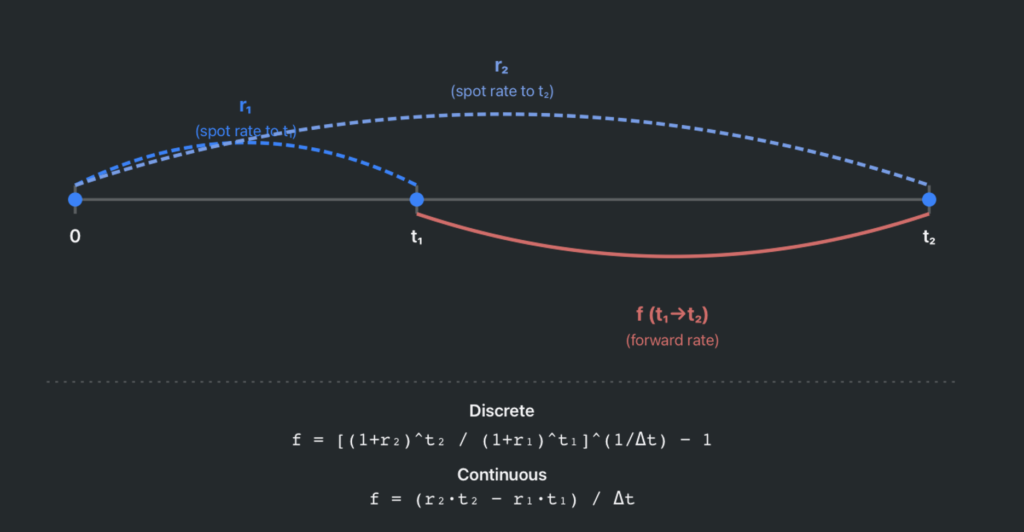
Defining the Forward Rate
Let denote the forward rate contracted today for an investment that begins at time and matures at time . The critical distinction from a spot rate is the investment period. A spot rate represents the return from now to time . A one-year forward rate represents the return between time and , also contracted today. The rate is locked in at the present moment, even though the investment period lies in the future.
To make this concrete: while a ten-year spot rate indicates the annualized return over ten years measured from today, the one-year forward rate in nine years’ time () isolates the return on a one-year investment specifically in the tenth year. The forward rate curve traces out these successive single-period returns across the term structure.
Deriving Forward Rates from Spot Rates
The no-arbitrage principle links spot and forward rates. An investor choosing between (a) investing for two years at the two-year spot rate, or (b) investing for one year at the one-year spot rate and then rolling into a one-year forward rate, must earn the same total return. Otherwise, a risk-less profit opportunity would exist. Formally:
Solving for the implied one-year forward rate one year from now:
Why Forward Rates Matter
For quantitative practitioners, forward rates serve several distinct purposes:
- Bond pricing: Discounting each cash flow by the product of sequential forward rates is mathematically equivalent to discounting by the corresponding spot rate, but offers finer granularity for risk analysis.
- Relative value analysis: Comparing implied forward rates to your own rate forecasts reveals potential mispricings.
- Derivative valuation: Forward Rate Agreements (FRAs), interest rate swaps, and other derivatives are priced directly off the forward curve.
One important caveat: implied forward rates are not forecasts. They reflect the rates that must hold for arbitrage-free pricing to be internally consistent. Whether they predict actual future rates depends on which term structure theory you subscribe to—pure expectations, liquidity preference, or market segmentation. For pricing purposes, however, this distinction is irrelevant: the forward rates embedded in today’s curve are the rates the market uses to value future cash flows.
The Relationship Between Spot Rates and Forward Rates: A Practical Example
We’ve now defined spot rates and forward rates individually. In this section, we connect them explicitly—showing how one determines the other and working through a numerical example you can verify yourself.
The Fundamental Link
The no-arbitrage condition requires that compounding the sequence of one-period forward rates produces the same total return as investing at the corresponding spot rate:
In other words, the t-period spot rate is the geometric average of the first t forward rates. This ensures no risk-less profit opportunity exists between holding a long-term zero-coupon bond and rolling over a series of shorter-term investments.
Rearranging to isolate a single forward rate:
This formula lets you extract any one-period forward rate from two adjacent spot rates.
A Worked Example
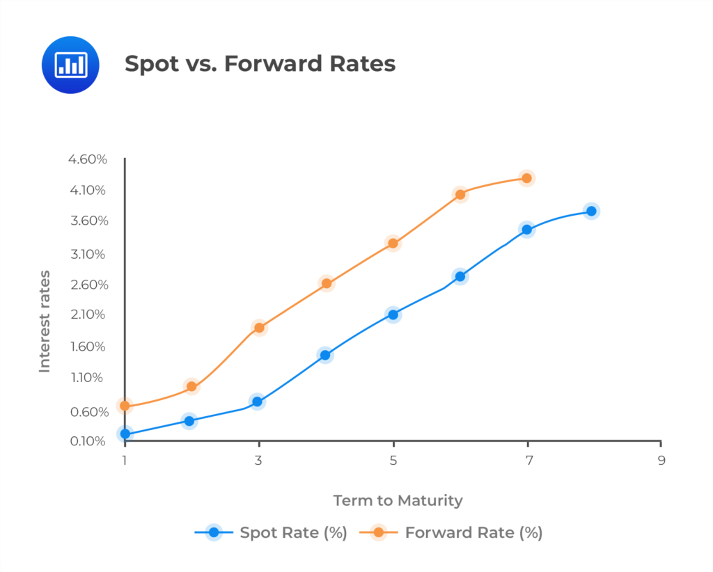
Suppose you observe the following spot rates: . The implied one-year forward rates are:
- = 4.00% (the one-year spot rate itself—there is no “earlier” rate to differentiate from)
- = ≈ 6.01%
- = ≈ 6.51%
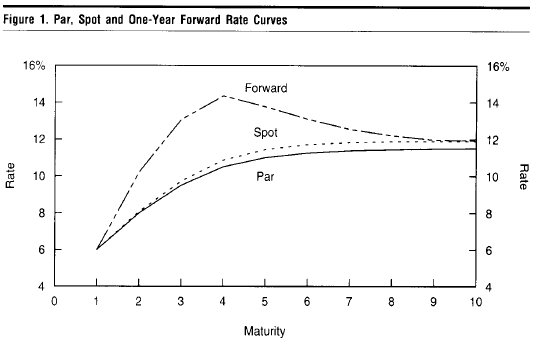
Notice how the forward rates exceed the spot rates when the spot curve is upward-sloping. This is not coincidental—it is a mathematical consequence of the compounding relationship. The spot rate at maturity is a blended average of all forward rates up to ; for the average to keep rising, each new forward rate must exceed the current average.
Python Code to Compute Forward Rates from a Given Spot Rate Curve
"""
Implied Forward Rates from Spot Rates
======================================
Computes one-period implied forward rates from a vector of spot rates.
"""

def implied_forward_rates(
    spot_rates: list[float],
    maturities: list[float] | None = None,
) -> list[float]:
    """
    Compute one-period implied forward rates from a vector of spot rates.

    Parameters
    ----------
    spot_rates : list[float]
        Annualised spot rates indexed by maturity (e.g. [r_1, r_2, ..., r_n]).
        Values should be in decimal form (0.05 = 5 %).
    maturities : list[float] | None
        Maturity of each spot rate in years.  Defaults to [1, 2, …, n].
        Useful for non-integer or irregular tenors (e.g. 0.5, 1, 2, 5).

    Returns
    -------
    list[float]
        One-period forward rates f(t₁→t₂) for consecutive maturity pairs.
        Length is len(spot_rates) - 1.

    Raises
    ------
    ValueError
        If fewer than two spot rates are supplied, or if maturities length
        does not match spot_rates.

    Examples
    --------
    >>> rates = [0.03, 0.035, 0.04, 0.044, 0.047]
    >>> implied_forward_rates(rates)
    [0.04003, 0.05012, 0.05616, 0.05913]  # approx

    Notes
    -----
    The forward rate f(t₁→t₂) is the breakeven rate that makes investing at
    the t₂-year spot rate equivalent to rolling over the t₁-year spot rate
    and then locking in f for the remaining (t₂-t₁) period.
    """
    n = len(spot_rates)

    if n < 2:
        raise ValueError("At least two spot rates are required.")

    if maturities is None:
        maturities = list(range(1, n + 1))  # 1, 2, 3, …, n (years)
    elif len(maturities) != n:
        raise ValueError(
            f"Length of maturities ({len(maturities)}) must match "
            f"length of spot_rates ({n})."
        )

    forwards: list[float] = []

    for i in range(n - 1):
        t1, t2 = maturities[i], maturities[i + 1]
        r1, r2 = spot_rates[i], spot_rates[i + 1]
        dt = t2 - t1  # length of the forward period

        if dt <= 0:
            raise ValueError(
                f"Maturities must be strictly increasing: "
                f"got t={t1} then t={t2}."
            )

        # Solve: (1+r2)^t2 = (1+r1)^t1 · (1+f)^dt
        growth_long  = (1 + r2) ** t2
        growth_short = (1 + r1) ** t1
        f = (growth_long / growth_short) ** (1 / dt) - 1

        forwards.append(round(f, 8))

    return forwards


# ── Demo ──────────────────────────────────────────────────────────────────────
if __name__ == "__main__":
    # Standard upward-sloping yield curve
    spot_rates   = [0.030, 0.035, 0.040, 0.044, 0.047]
    maturity_yrs = [1.,     2.,     3.,     4.,     5.    ]

    print("=" * 52)
    print(f"{'Maturity':<12}{'Spot Rate':>12}{'Forward Rate':>16}")
    print("-" * 52)

    for i, (t, r) in enumerate(zip(maturity_yrs, spot_rates)):
        print(f"{t:<12}{r:>11.3%}", end="")
        if i == 0:
            print(f"{'(base)':>16}")
        else:
            fwd = implied_forward_rates(
                spot_rates[:i+1],
                maturities=maturity_yrs[:i+1]
            )[-1]
            print(f"{fwd:>15.3%}")

    print("=" * 52)

    # Irregular tenors — e.g. 6m, 1y, 2y, 5y, 10y
    print("\nIrregular tenors (0.5, 1, 2, 5, 10):")
    irr_spots = [0.04, 0.042, 0.046, 0.052, 0.055]
    irr_mats  = [0.5,  1.0,   2.0,   5.0,   10.0 ]
    irr_fwds  = implied_forward_rates(irr_spots, maturities=irr_mats)
    for (t1, t2), f in zip(zip(irr_mats, irr_mats[1:]), irr_fwds):
        print(f"  f({t1}→{t2}): {f:.4%}")

# Output:
"""
====================================================
Maturity       Spot Rate    Forward Rate
----------------------------------------------------
1.0              3.000%          (base)
2.0              3.500%         4.002%
3.0              4.000%         5.007%
4.0              4.400%         5.609%
5.0              4.700%         5.909%
====================================================

Irregular tenors (0.5, 1, 2, 5, 10):
  f(0.5→1.0): 4.4004%
  f(1.0→2.0): 5.0015%
  f(2.0→5.0): 5.6019%
  f(5.0→10.0): 5.8009%
"""Practical Implications
This relationship has direct applications across fixed-income analytics:
- Bond pricing: You can price a coupon bond by discounting each cash flow at the corresponding spot rate, or equivalently, by discounting through the chain of forward rates. Both approaches yield the same price—a useful consistency check in any implementation.
- Scenario analysis: Shifting individual forward rates lets you stress-test a portfolio’s sensitivity to rate changes at specific future periods.
- Stochastic modeling: In the Heath-Jarrow-Morton (HJM) framework, the dynamics of drive the evolution of the entire yield curve, making forward rates the natural state variables for term structure models.
Grasping this spot-forward linkage gives you the algebraic scaffolding on which nearly all fixed-income analytics are built. Next, we’ll see how to extract these rates from real market data.
Bootstrapping the Yield Curve: A Step-by-Step Walkthrough
Markets do not hand you a clean set of spot rates. Instead, you observe prices of coupon-bearing bonds across various maturities and must extract the underlying zero-coupon (spot) rates yourself. This extraction process is called bootstrapping, and it builds the spot rate curve iteratively—one maturity at a time.
The Core Idea
Each coupon bond’s price equals the sum of its discounted cash flows. If you already know the spot rates for shorter maturities, you can solve for the single unknown spot rate at the next maturity. By starting from the shortest-maturity instrument and working outward, you bootstrap the entire term structure.
A Concrete Example
Suppose you observe three par bonds (price = 100) with annual coupons:
| Maturity | Coupon Rate | Price |
|---|---|---|
| 1 year | 4.00% | 100 |
| 2 years | 4.80% | 100 |
| 3 years | 5.50% | 100 |
Step 1 — Solve for . The 1-year bond pays a single cash flow of 104 at year-end. Setting price equal to discounted value:
Step 2 — Solve for . The 2-year bond pays a 4.80 coupon at year 1 and 104.80 at year 2. Using the we just found:
Compute the first term (≈ 4.6154), subtract from 100, and solve for . This yields ≈ 4.8116%.
Step 3 — Solve for . The 3-year bond pays coupons of 5.50 at years 1 and 2, plus 105.50 at year 3. Discount the first two cash flows with and , then solve for :
This yields ≈ 5.5358%.
Notice that spot rates diverge slightly from coupon rates as maturity increases—a direct consequence of the reinvestment assumptions embedded in par yields versus zero-coupon rates.
Python Implementation for Bootstrapping the Yield Curve
The algorithm generalizes cleanly for programmatic use:
def bootstrap_spot_rates(bonds):
    """
    Computes spot rates using the bootstrapping method.

    Args:
        bonds: List of tuples (maturity, coupon_rate, price)
               Example: [(1, 0.05, 101), (2, 0.06, 102)]

    Returns:
        Dictionary mapping maturity (int) to spot rate (float).
    """
    # Sort bonds by maturity to ensure we solve iteratively
    sorted_bonds = sorted(bonds, key=lambda x: x[0])
    spot_rates = {}

    for maturity, coupon_rate, price in sorted_bonds:
        coupon = coupon_rate * 100

        # If maturity is 1, it's a simple zero-coupon calculation (or 1-period bond)
        if maturity == 1:
            # P = (C + 100) / (1 + z1)
            z = (coupon + 100) / price - 1
            spot_rates[1] = z
        else:
            # Calculate the PV of all coupons prior to maturity
            # using existing spot rates
            pv_coupons = 0
            for t in range(1, maturity):
                if t not in spot_rates:
                    raise ValueError(f"Missing spot rate for year {t}. Bootstrapping requires a continuous curve.")

                pv_coupons += coupon / ((1 + spot_rates[t]) ** t)

            # Solve for the spot rate at current maturity
            # Price = pv_coupons + (coupon + 100) / (1 + zn)^n
            remaining_pv = price - pv_coupons

            if remaining_pv <= 0:
                raise ValueError(f"Invalid bond data at maturity {maturity}: PV of final payment is non-positive.")

            z = ((coupon + 100) / remaining_pv) ** (1 / maturity) - 1
            spot_rates[maturity] = z

    return spot_rates


if __name__ == "__main__":
    # Data format: (Maturity, Annual Coupon Rate, Market Price)
    bond_data = [
        (1, 0.03, 101.50),  # 1-yr bond, 3% coupon, price 101.50
        (2, 0.04, 102.10),  # 2-yr bond, 4% coupon, price 102.10
        (3, 0.05, 103.40)   # 3-yr bond, 5% coupon, price 103.40
    ]

    try:
        rates = bootstrap_spot_rates(bond_data)
        print("Maturity | Spot Rate")
        print("-" * 20)
        for year, rate in rates.items():
            print(f"{year:8} | {rate:.4%}")
    except ValueError as e:
        print(f"Error: {e}")

# Output:
"""
Maturity | Spot Rate
--------------------
       1 | 1.4778%
       2 | 2.9327%
       3 | 3.8485%
"""Why This Matters
Bootstrapping gives you the discount factors needed to price any fixed-income instrument consistently—not just the bonds you started with. Once you have the spot curve, deriving forward rates is a direct application of the formulas from the previous sections, and you can value swaps, structured products, or any arbitrary cash flow schedule without relying on a single yield-to-maturity approximation. For data scientists building pricing engines or risk models, bootstrapping is the essential bridge from observed market data to a usable term structure.
Bringing It All Together
Throughout this post, we’ve built up the three foundational pillars of fixed-income pricing: the term structure of interest rates, spot rates, and forward rates. Here’s how they connect.
Traditional bond pricing relies on a single discount rate—such as the yield-to-maturity—applied uniformly to all future cash flows. This is a simplifying assumption. In reality, interest rates vary with time-to-maturity, and the term structure captures exactly this variation. Recognizing this fact moves us from a flat discounting model to a more granular, accurate pricing framework.
Spot rates serve as the building blocks. Each spot rate represents the annualized yield on a zero-coupon instrument maturing at time , contracted today. When you discount a bond’s cash flows, each payment at time gets its own discount factor:
This per-maturity discounting eliminates the distortion introduced by applying a single flat rate across all maturities.
Forward rates emerge naturally from the spot rate curve. A one-year forward rate represents the implied return between time and , locked in today. The no-arbitrage relationship binds them:
Under the expectations hypothesis, forward rates equal the market’s expected future spot rates—i.e., equals the one-year spot rate expected to prevail in year two. While this hypothesis is elegant and intuitive, real markets incorporate risk premia, so forward rates don’t purely reflect expectations.
Here’s a concise summary of the relationships:
- Term structure → the full curve of yields across maturities
- Spot rates → zero-coupon yields for each specific maturity, extracted (bootstrapped) from observable bond prices
- Forward rates → implied future rates derived from adjacent spot rates via no-arbitrage conditions
Why This Matters for Quantitative Practitioners
For data scientists and ML engineers working in finance, these concepts form the input layer for virtually every fixed-income model. Whether you’re building a pricing engine, training a model to predict yield curve movements, or constructing a risk management system, you need to correctly extract spot rates, compute forward rates, and understand what the term structure is telling you. Misapplying a flat discount rate where a full term structure is warranted introduces systematic pricing errors—errors that compound across large portfolios.
The mathematical framework here is deliberately straightforward: it relies on algebraic manipulation and basic compounding. Yet its implications are profound. Mastering these relationships equips you to move confidently into more advanced territory—swap pricing, duration and convexity analysis, interest rate derivatives, and stochastic term structure models like Heath-Jarrow-Morton and Hull-White. The spot-forward relationship is the grammar of fixed income; everything else is built on it.
Frequently Asked Questions
Q: What is the term structure of interest rates?
A: The term structure of interest rates describes the relationship between interest rates (or yields) and their corresponding maturities. It is typically visualized as the yield curve, which plots annualized yields of zero-coupon bonds against their time to maturity. The shape of the curve—normal, inverted, or flat—reflects market expectations about future rates, risk premiums, and economic conditions.
Q: What is the difference between a spot rate and a forward rate?
A: A spot rate is the annualized yield on a zero-coupon bond from today to a specific future maturity, representing the cost of borrowing or lending over that single period. A forward rate, by contrast, is an implied future interest rate derived from two spot rates, representing the market’s expected rate between two future dates. Forward rates are extracted from the spot curve using no-arbitrage relationships.
Q: How does bootstrapping the yield curve work?
A: Bootstrapping is a sequential method for extracting spot rates from observed market prices of coupon-bearing bonds. Starting with the shortest maturity instrument, you solve for each spot rate one at a time, using previously derived spot rates to discount earlier cash flows. This iterative process builds a complete zero-coupon yield curve that is consistent with observed bond prices.
Q: Why can’t you use a single discount rate to price all bonds?
A: A single flat discount rate assumes that interest rates are identical across all maturities, which almost never holds in practice. Short-term and long-term bonds carry different yields due to factors like interest rate expectations, liquidity preferences, and risk premiums. Using maturity-specific spot rates from the term structure ensures accurate, no-arbitrage bond pricing that reflects real market conditions.
Q: What is a discount factor and how does it relate to spot rates?
A: A discount factor is the present value of one unit of currency to be received at a specific future date. It is directly derived from the spot rate for that maturity: for a spot rate r over t years, the discount factor equals 1/(1+r)^t. Discount factors are the building blocks of bond pricing, as multiplying each future cash flow by its corresponding discount factor and summing the results gives the bond’s fair price.