Why Bond Pricing Matters in Quantitative Finance
In quantitative finance, accurately pricing a bond is not merely an academic exercise—it is a foundational skill that underpins portfolio valuation, risk management, interest rate modeling, and derivatives pricing. Whether you are building a fixed-income analytics engine, backtesting a trading strategy, or constructing a yield curve, understanding how bond prices relate to yields is essential.
At its core, bond pricing answers a deceptively simple question: what is the present value of a bond’s future cash flows? A bond promises its holder a series of periodic coupon payments and a final return of face value (par) at maturity. The price of the bond is the sum of these cash flows, each discounted back to the present using an appropriate rate. That rate, the Yield to Maturity (YTM), is the single, uniform discount rate that equates the bond’s discounted future cash flows to its current market price.
YTM as the Internal Rate of Return
YTM functions as the bond’s internal rate of return (IRR). It represents the estimated annual rate of return an investor can expect if they purchase the bond at its current price, hold it until maturity, and reinvest all coupon payments at the same rate. This “promised yield” rests on three critical assumptions:
- The investor holds the bond to maturity (no early sale).
- The issuer does not default on any scheduled payments.
- All interim coupon payments are reinvested at the YTM itself.
These assumptions simplify the model considerably, but they also introduce limitations that practitioners must account for in real-world applications—particularly when modeling credit risk or interest rate volatility.
Why It Matters for Practitioners
For data scientists and developers entering financial modeling, bond pricing with YTM serves as a gateway to deeper concepts: duration, convexity, term structure modeling, and option-adjusted spreads. The math is tractable, the intuition is transferable, and the implementation lends itself naturally to programmatic solutions.
Consider a simple scenario: a bond with a known face value, coupon rate, and maturity date is trading at a market price. Computing the YTM requires solving for the discount rate in a present value equation—a root-finding problem that maps directly to numerical methods you likely already use.
Throughout this post, we will formalize this relationship, derive the pricing formula, implement it in code, and explore how changes in yield affect bond prices. By the end, you will have both the mathematical framework and a working implementation to price fixed-income securities confidently.
Bond Basics: Key Terminology, Components, and Cash Flow Structure
Before diving into yield-to-maturity calculations and pricing models, you need a firm grasp of the fundamental building blocks that define a bond. At its core, a bond is a debt instrument—a contract in which an issuer (borrower) promises to pay a bondholder (lender) a series of cash flows over a specified period.
Core Terminology
Every bond is characterized by a handful of key parameters:
- Face Value (Par Value): The principal amount the issuer repays at maturity, typically $1,000 for corporate and government bonds. This serves as the baseline for calculating coupon payments.
- Coupon Rate: The fixed annual interest rate applied to the face value to determine periodic interest payments. A bond with a 5% coupon rate and $1,000 face value pays $50 per year.
- Maturity Date: The date on which the issuer returns the face value to the bondholder, terminating the contract.
- Market Price: The current trading price of the bond, which may differ from par value depending on prevailing interest rates, credit risk, and time to maturity.
- Yield to Maturity (YTM): The internal rate of return an investor earns by purchasing the bond at its current market price and holding it until maturity, assuming all coupon payments are reinvested at the same rate and the issuer does not default. YTM is often used interchangeably with the term market discount rate.
Cash Flow Structure
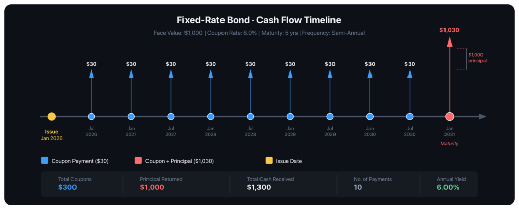
A standard fixed-rate bond generates two types of cash flows: periodic coupon payments and a lump-sum principal repayment at maturity. For a semi-annual coupon bond—the most common convention in U.S. markets—each coupon payment equals half the annual coupon amount, and payments occur every six months.
Consider a concrete example: a 3-year bond with a $1,000 face value and a 6% annual coupon, paid semi-annually. The cash flow timeline looks like this:
Time (periods):   1     2     3     4     5     6
Cash Flows ($):  30    30    30    30    30   1030
Periods 1 through 5 each deliver a $30 coupon payment ($1,000 × 6% / 2). At period 6, the bondholder receives the final coupon plus the face value, totaling $1,030.
Why This Matters for Pricing
Bond pricing reduces to a single operation: discounting each future cash flow back to the present using an appropriate rate. That rate is the YTM. When the YTM equals the coupon rate, the bond trades at par. When the YTM exceeds the coupon rate, the bond trades at a discount; when it falls below, the bond trades at a premium.
Understanding this cash flow structure is essential because every pricing formula, numerical solver, and sensitivity analysis you will encounter builds directly on top of it. A bond is, in effect, a deterministic sequence of cash flows—making it an ideal starting point for quantitative modeling.
With these fundamentals established, we can now formalize the mathematical relationship between price, cash flows, and yield.
Understanding Yield to Maturity: Definition, Intuition, and the IRR Connection
Yield to maturity (YTM) represents the total annualized rate of return an investor can expect by holding a bond until its maturity date, assuming all coupon payments are reinvested at the same rate. In precise terms, YTM is the bond’s internal rate of return (IRR)—the single, uniform discount rate that equates the present value of all future cash flows (coupons plus face value) to the bond’s current market price.
This definition deserves unpacking.
The IRR Connection
If you have worked with discounted cash flow (DCF) analysis in any context—project valuation, startup modeling, or portfolio assessment—you already understand IRR intuitively. YTM applies the same concept to fixed-income securities. It solves for the rate in the following equation:
where is the current bond price, is the periodic coupon payment, is the face (par) value, and is the number of periods to maturity. There is no closed-form algebraic solution for —it must be found numerically, which is why YTM and IRR are computationally identical problems.
Key Assumptions
YTM carries three assumptions that practitioners must keep in mind:
- The investor holds the bond to maturity. Any early sale introduces price risk driven by prevailing interest rates at the time of sale.
- All coupon payments are reinvested at the YTM rate. In practice, reinvestment rates fluctuate, making this an idealization rather than a guarantee.
- The issuer does not default. YTM is often called the bond’s promised yield precisely because it assumes full and timely payment of all obligations.
These assumptions mean YTM functions as a theoretical benchmark—powerful for comparing bonds on a level playing field, but not a literal forecast of realized return.
Intuition for Practitioners
Think of YTM as the bond market’s way of compressing a complex stream of cash flows into a single, comparable number. When you see a bond quoted at a 5.2% yield, the market is telling you: “At the current price, if every assumption holds, you earn 5.2% annualized.” This figure is also referred to as the market discount rate or the implied yield, reflecting the rate the market collectively demands for that bond’s risk and duration profile.
For data scientists and developers building pricing engines, YTM is the critical input that bridges observable market prices and theoretical valuations. Understanding it deeply—and understanding its limitations—is the foundation upon which more sophisticated models (spread analysis, option-adjusted yield, term structure fitting) are built.
Now that we have a clear conceptual grasp of YTM, let’s formalize the pricing formula and examine the inverse relationship between price and yield.
The Bond Pricing Formula: Deriving Price from YTM and the Inverse Price-Yield Relationship
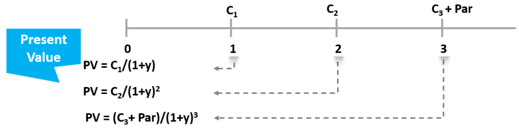
With the concept of YTM established, we can now formalize the pricing equation. The bond pricing formula expresses a bond’s present value as the sum of its discounted future cash flows, where the discount rate is the yield to maturity.
The Core Formula
For a fixed-rate bond paying periodic coupons, the price is:
where is the periodic coupon payment, is the face (par) value, is the YTM per period, and is the total number of periods to maturity. The first term represents the present value of the annuity stream of coupon payments; the second captures the discounted redemption value at maturity.
Consider a concrete example: a 5-year bond with a face value of $1,000, a 6% annual coupon, and a YTM of 8%.
Each $60 coupon and the final $1,000 principal are discounted at 8%. The resulting price falls below par—approximately $920.15—because the market demands a higher return than the coupon provides. This bond trades at a discount.
The Inverse Price-Yield Relationship
A fundamental property emerges directly from the formula: bond prices move inversely to yields. When increases, the denominators grow larger, compressing the present value of every future cash flow. When decreases, those denominators shrink, inflating the price.
This relationship produces three canonical pricing states:
- Par: Price equals face value when YTM equals the coupon rate.
- Discount: Price falls below par when YTM exceeds the coupon rate.
- Premium: Price rises above par when YTM is less than the coupon rate.
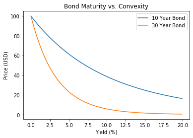
Critically, the price-yield curve is convex, not linear. A 1% decrease in yield raises the price by more than a 1% increase in yield lowers it. This asymmetry—convexity—has significant implications for hedging and portfolio risk management that practitioners must internalize.
Why This Matters Computationally
From a modeling perspective, the pricing formula is straightforward to implement. However, solving the inverse problem—extracting YTM from an observed market price—requires numerical methods. No closed-form solution exists for when . Practitioners typically apply Newton-Raphson iteration or bisection search to converge on the yield that satisfies the pricing equation. Understanding the analytical structure of the formula makes implementing these solvers both more efficient and more robust.
Let’s put this theory into practice with step-by-step calculations across all three pricing states.
Worked Examples: Step-by-Step Bond Price Calculations for Discount, Premium, and Par Bonds
To solidify the pricing mechanics, let’s walk through three canonical scenarios using the same bond structure with different yield assumptions.
Setup and Formula
Consider a bond with face value , annual coupon rate , maturity of and market YTM of . The price is:
where is the annual coupon payment.
Par Bond: Coupon Rate = YTM
When the coupon rate equals the market yield, the bond prices at par. Set .
- Annual coupon: $50
- Price = $50/(1.05)¹ + $50/(1.05)² + $50/(1.05)³ + $1,000/(1.05)³
- Price = $47.62 + $45.35 + $43.19 + $863.84 = $1,000.00
The result confirms the identity: when the coupon rate matches YTM, the bond trades at exactly face value.
Discount Bond: Coupon Rate < YTM
Now raise the required yield to while keeping
- Price = $50/(1.07)¹ + $50/(1.07)² + $50/(1.07)³ + $1,000/(1.07)³
- Price = $46.73 + $43.67 + $40.81 + $816.30 = $947.51
The bond sells below par because investors demand a higher return than the coupon provides. The market compensates by lowering the price, creating a built-in capital gain at maturity.
Premium Bond: Coupon Rate > YTM
Finally, set with the same
- Price = $50/(1.03)¹ + $50/(1.03)² + $50/(1.03)³ + $1,000/(1.03)³
- Price = $48.54 + $47.13 + $45.76 + $915.14 = $1,056.57
Here the coupon exceeds the market rate, so investors pay a premium. The price exceeds face value, embedding a capital loss at maturity that offsets the above-market coupon income.
Implementation Reference
# compute bond price given YTM, coupon rate, face value, and maturity
def bond_price(face, coupon_rate, ytm, n):
    coupon = face * coupon_rate
    pv_coupons = sum(coupon / (1 + ytm)**t for t in range(1, n + 1))
    pv_face = face / (1 + ytm)**n
    return pv_coupons + pv_face

# Par, Discount, Premium
print(bond_price(1000, 0.05, 0.05, 3))  # 1000.00
print(bond_price(1000, 0.05, 0.07, 3))  # 947.51
print(bond_price(1000, 0.05, 0.03, 3)) # 1056.57The key takeaway is mechanical yet powerful: the relationship between coupon rate and YTM entirely determines whether a bond trades at par, at a discount, or at a premium. This inverse relationship between yield and price is the foundational dynamic of fixed-income markets—and the starting point for more advanced analytics like duration and convexity.
With the pricing formula validated across all three states, let’s turn to the computational challenge of solving the inverse problem: given a market price, how do we extract the YTM?
Implementing Bond Pricing in Python: From Approximation Formula to Numerical YTM Solver
Computing YTM from a bond’s market price requires solving a nonlinear equation—making it a natural candidate for Python implementation. In this section, we build two complementary tools: a fast approximation for quick estimation and a precise numerical solver for production use.
The Approximation Formula
Before reaching for a numerical solver, practitioners often use a quick approximation to estimate YTM:
where C is the annual coupon payment, F is the face (par) value, P is the current market price, and N is the number of years to maturity. This formula averages the annual coupon income with the annualized capital gain or loss, then divides by the midpoint of face value and price. It typically lands within 10–30 basis points of the true YTM for plain-vanilla bonds.
# Implementation of the YTM approximation formula
def approximate_ytm(price, face_value, coupon_rate, years):
    """
    Calculates the approximate Yield to Maturity (YTM) for a bond.

    price: Current market price (PV)
    face_value: Par value of the bond (FV)
    coupon_rate: Annual coupon rate as a decimal (e.g., 0.05 for 5%)
    years: Number of years until maturity (n)
    """
    annual_coupon = face_value * coupon_rate
    numerator = annual_coupon + (face_value - price) / years
    denominator = (face_value + price) / 2
    return numerator / denominator

# Example: $947.51 price, $1000 face value, 5% coupon, 5 years to maturity
ytm = approximate_ytm(947.51, 1000, 0.05, 5)
print(f"Approximate YTM: {ytm:.2%}") # Approximate YTM: 6.21%

# Example: $1056.57 price, $1000 face value, 5% coupon, 5 years to maturity
ytm = approximate_ytm(1056.57, 1000, 0.05, 5)
print(f"Approximate YTM: {ytm:.2%}") # Approximate YTM: 3.76%

# Example: $950 price, $1000 face value, 6% coupon, 5 years to maturity
ytm = approximate_ytm(950, 1000, 0.06, 5)
print(f"Approximate YTM: {ytm:.2%}") # Approximate YTM: 7.18%The Exact Bond Price Equation
The exact relationship between price and yield is the present-value identity:
Given a known price P, solving for y (the YTM) analytically is impossible for most maturities because the equation is a polynomial of degree N. This is where numerical methods become essential.
Building a Numerical YTM Solver
Python’s scipy.optimize module provides robust root-finding algorithms. The approach is straightforward: define a function that returns the difference between the theoretical bond price at a candidate yield and the observed market price, then let brentq (or newton) find the root.
import scipy.optimize as optimize

def bond_ytm(price, par, T, coup, freq=2, guess=0.05):
    """
    Calculate the Yield to Maturity (YTM) of a bond.
    """
    freq = float(freq)
    periods = T * freq
    coupon = coup / 100. * par / freq
    dt = [(i + 1) / freq for i in range(int(periods))]

    # Calculate price based on a yield y
    ytm_func = lambda y: \
        sum([coupon / (1 + y / freq)**(freq * t) for t in dt]) + \
        par / (1 + y / freq)**(freq * T) - price

    # Use Newton's method to find the root
    return optimize.newton(ytm_func, guess)

# Example Usage:
# Price=950, Par=1000, T=5 years, Coupon=6%, Freq=1
ytm = bond_ytm(95.0428, 100, 1.5, 5.75, 2)
print(f"YTM: {ytm:.4f}")
# Output: YTM: 0.0723 (7.23%)For a 5-year bond with a 6% annual coupon, $1,000 face value, and a market price of $950, the approximation formula returns roughly 7.18%, while the numerical solver converges to approximately 7.23%. The small gap confirms the approximation’s utility for quick screening, but the solver delivers the precision required for trading desks and risk models.
Key Takeaways
- Use the approximation for rapid estimation and sanity checks.
- Use the numerical solver when basis-point accuracy matters—pricing, hedging, and portfolio analytics all demand it.
- Wrapping both approaches in reusable Python functions lets you validate one against the other, catching implementation errors early.
This two-pronged approach—fast estimate plus precise solver—mirrors how quantitative practitioners actually work: intuition first, then rigor.
From Theory to Practice – Assumptions, Limitations, and Next Steps
The bond pricing framework built around Yield to Maturity offers an elegant, tractable model—but like any model, it rests on assumptions that practitioners and developers must understand before deploying it in production systems.
Key Assumptions Behind YTM
Recall that YTM is the single, uniform discount rate that equates the present value of all future cash flows to the bond’s current market price. This definition implicitly carries three critical assumptions:
- The investor holds the bond until maturity. Any early sale exposes the investor to price risk driven by interest rate movements, meaning the realized return may diverge significantly from the computed YTM.
- All coupon payments are reinvested at the YTM rate. In practice, prevailing market rates fluctuate, and reinvestment at the exact YTM is rarely achievable. This reinvestment risk is one of the most frequently overlooked sources of error in naive yield comparisons.
- The issuer does not default. YTM is a “promised yield” that assumes full and timely payment of all coupons and principal. Credit risk is entirely absent from the calculation.
Practical Limitations for Quantitative Work
For data scientists and developers building pricing engines, these assumptions translate into concrete modeling gaps. A flat discount rate across all maturities ignores the term structure of interest rates—the reality that short-term and long-term rates differ. A more robust approach uses a full yield curve (spot rates or zero-coupon rates) to discount each cash flow individually, rather than applying a single YTM uniformly.
Additionally, the YTM calculation itself requires numerical methods—Newton-Raphson, bisection, or Brent’s method—to solve iteratively. If you implemented the solver in the previous section, you have already encountered this firsthand.
Edge cases matter too. Bonds with embedded options (callable or putable bonds), floating-rate coupons, or irregular payment schedules all break the standard YTM framework and require adjusted metrics like yield to call or option-adjusted spread (OAS).
Next Steps
With a solid grasp of flat-rate bond pricing, you are well positioned to explore several natural extensions:
- Bootstrapping the yield curve from observable bond prices to extract spot rates.
- Duration and convexity — first- and second-order sensitivities of bond price to yield changes.
- Credit spread modeling to relax the no-default assumption.
- Monte Carlo simulation of interest rate paths for portfolio-level risk analysis.
Each of these builds directly on the pricing mechanics covered here. The YTM framework is not the final word but the foundation. Treat it as a baseline model: invaluable for intuition and quick estimation, but insufficient on its own for rigorous fixed-income analytics. Understanding exactly where it breaks down is what separates a textbook implementation from a production-grade one.
Frequently Asked Questions
Q: What is yield to maturity (YTM) in bond pricing?
A: Yield to maturity (YTM) is the single, uniform discount rate that equates a bond’s current market price to the present value of all its future cash flows, including coupon payments and the return of par value at maturity. It represents the total annualized return an investor would earn if the bond is held until maturity and all payments are reinvested at the same rate.
Q: How do you calculate the price of a coupon bond using the present value of cash flows?
A: A coupon bond’s price is calculated by discounting each future cash flow—periodic coupon payments and the final par value—back to the present using the yield to maturity as the discount rate. The bond price equals the sum of each coupon payment divided by (1 + YTM)^t for each period t, plus the par value divided by (1 + YTM)^n, where n is the total number of periods.
Q: Why does a bond trade at a discount or premium to par value?
A: A bond trades at a discount when its coupon rate is lower than the prevailing market yield (YTM), meaning investors demand a lower price to compensate for below-market interest payments. Conversely, a bond trades at a premium when its coupon rate exceeds the market yield, making its higher cash flows more valuable. When the coupon rate equals the YTM, the bond trades at par.
Q: How can you implement bond pricing in Python?
A: Bond pricing in Python can be implemented by defining a function that takes par value, coupon rate, YTM, and maturity as inputs, then iterates over each period to compute the present value of coupon payments and adds the discounted par value. Libraries such as NumPy and SciPy can be used for efficient vectorized calculations and for solving the inverse problem of finding YTM from a given price.
Q: What is the relationship between bond prices and interest rates?
A: Bond prices and interest rates have an inverse relationship: when market interest rates rise, existing bond prices fall because their fixed cash flows become less attractive relative to new bonds issued at higher rates. When rates decline, existing bond prices increase. This relationship is a direct consequence of the time value of money and the discounting mechanism used in fixed income valuation.