Why Measuring Text Similarity Matters
In virtually every domain where unstructured text plays a role—search engines ranking documents against a query, recommendation systems surfacing relevant content, plagiarism detectors flagging duplicate submissions—there lies a fundamental computational challenge: how do you quantify the similarity between two pieces of text? Natural language is inherently high-dimensional, ambiguous, and context-dependent. Reducing it to a measurable, comparable representation is non-trivial, yet it underpins some of the most critical pipelines in modern NLP and information retrieval.
The Core Problem: From Words to Numbers
Text, in its raw form, is incompatible with mathematical operations. Before any similarity computation can occur, documents must be transformed into vector representations. Each unique term in a corpus defines a dimension, and the frequency or weight (e.g., TF-IDF) of that term within a given document populates the corresponding component of its vector. The result is a high-dimensional, typically sparse vector space where each document occupies a specific point—or more precisely, a specific direction.
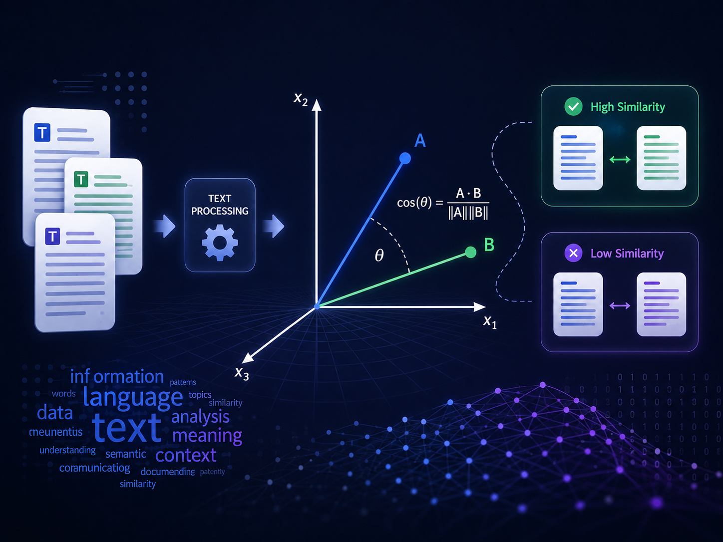
This transformation introduces a key question: once you have two vectors, what metric best captures their semantic proximity? Euclidean distance is an intuitive choice, but it conflates magnitude with orientation. A longer document and a shorter document discussing identical topics would appear distant in Euclidean space simply due to differences in term frequency totals. This is where cosine similarity becomes indispensable.
Why Cosine Similarity Dominates Text Analysis
Cosine similarity measures the cosine of the angle between two vectors, effectively normalizing for magnitude and focusing exclusively on directional alignment. Two documents with identical term distributions but vastly different lengths will yield a cosine similarity of 1.0—perfect similarity—because the angle between them is zero. This magnitude invariance makes it particularly well-suited for text analysis, where document length varies widely and what matters is the proportion of shared concepts, not raw term counts.
Its advantages extend further:
- Efficient computation on sparse vectors: Text vectors in large corpora are overwhelmingly sparse (most terms appear in very few documents). Cosine similarity handles this sparsity gracefully, requiring only the non-zero overlapping dimensions for calculation.
- Bounded output range: The metric produces values in [−1, 1] (or [0, 1] for non-negative term weights), providing an immediately interpretable similarity score.
- Scalability: It integrates seamlessly with vectorized operations in libraries like NumPy and scikit-learn, enabling batch comparisons across millions of document pairs.
Known Limitations and Emerging Alternatives
Despite its dominance, cosine similarity is not without deficiencies. As recent research highlights, it yields identical values for vector pairs that share the same angle regardless of how different the vectors are in absolute magnitude—a property that can obscure meaningful distinctions in certain analytical contexts. Alternative metrics like the Vector Similarity Metric (VSM) have been proposed to address this gap by incorporating both angular and magnitude-based differences into a single score.
Additionally, cosine similarity operates on surface-level term overlap. It remains sensitive to lexical variation: synonyms receive no credit, and antonyms or negations can produce misleadingly high similarity scores when they share vocabulary. Modern embedding-based approaches (Word2Vec, BERT) mitigate this by projecting text into dense semantic spaces, but cosine similarity remains the go-to metric within those spaces for comparing the resulting vectors.
Setting the Stage
Understanding why text similarity measurement matters is the prerequisite for understanding how cosine similarity works at a mechanical level. Whether you are building a semantic search engine, clustering customer feedback, or deduplicating a dataset, the choice of similarity metric directly shapes the quality of your results. In the sections that follow, we will dissect the mathematics behind cosine similarity, implement it from scratch and with production-grade libraries, and critically evaluate when it excels—and when you should reach for something else.
The Math Behind Cosine Similarity: Vectors, Angles, and the Formula
At its core, cosine similarity measures the cosine of the angle between two non-zero vectors in a multi-dimensional space. Rather than computing the absolute distance between points—as Euclidean distance does—cosine similarity captures the orientation of vectors, making it magnitude-independent. This property is precisely what makes it indispensable in text analysis, where document length can vary dramatically but semantic similarity should remain consistent.
From Text to Vectors
Before applying cosine similarity, you must represent text as numerical vectors. Each unique word in a corpus defines a dimension, and the frequency (or TF-IDF weight) of that word within a given document determines the value along that dimension. Consider two short documents:
- Document A: “the cat sat on the mat”
- Document B: “the cat lay on the rug”
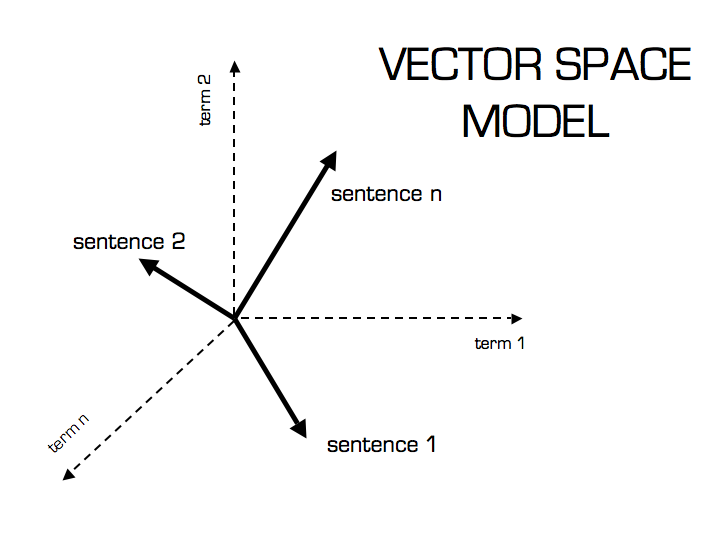
After tokenization and vocabulary construction, each document becomes a sparse vector in a high-dimensional space where most entries are zero. This transformation—often called the vector space model—is the foundational step that enables geometric reasoning over text.
# Convert two sample documents into TF-IDF vectors using
# scikit-learn's TfidfVectorizer
import pandas as pd
from sklearn.feature_extraction.text import TfidfVectorizer

# 1. Define sample documents
documents = [
    "the cat sat on the mat",
    "the cat lay on the rug"
]

# 2. Initialize the Vectorizer
vectorizer = TfidfVectorizer()

# 3. Fit and transform the documents
tfidf_matrix = vectorizer.fit_transform(documents)

# 4. Convert to a readable format (DataFrame)
feature_names = vectorizer.get_feature_names_out()
df = pd.DataFrame(tfidf_matrix.toarray(), columns=feature_names)

print(df)

# Output:
"""
        cat       lay       mat        on       rug       sat       the
0  0.317011  0.000000  0.445548  0.317011  0.000000  0.445548  0.634021
1  0.317011  0.445548  0.000000  0.317011  0.445548  0.000000  0.634021
"""The Formula
Given two vectors A and B, cosine similarity is defined as:
Breaking this down into its components:
- Dot product (A · B): The sum of element-wise products, . This captures how much the two vectors “agree” across each dimension.
- Magnitude (‖A‖): The L2 norm of the vector, . This normalizes each vector to unit length.
- Division: By dividing the dot product by the product of magnitudes, you effectively project both vectors onto the unit hypersphere, isolating directional similarity from scale.
The result falls within the range [-1, 1] for general vectors, though in text analysis—where term weights are non-negative—the range narrows to [0, 1]. A value of 1 indicates identical orientation (maximum similarity), 0 indicates orthogonality (no similarity), and values approaching -1 would indicate diametrically opposed directions (rare in standard text representations).
# Implementing cosine similarity from scratch using NumPy,
# showing dot product and norm calculations step by step
import numpy as np

# 1. Define two sample vectors (e.g., from TF-IDF)
vector_a = np.array([0.5, 0.8, 0.0, 0.1])
vector_b = np.array([0.4, 0.9, 0.2, 0.0])

def manual_cosine_similarity(a, b):
    # Step A: Calculate the Dot Product
    dot_product = np.dot(a, b)

    # Step B: Calculate the L2 Norm (Magnitude) of each vector
    norm_a = np.linalg.norm(a)
    norm_b = np.linalg.norm(b)

    # Step C: Divide dot product by the product of norms
    similarity = dot_product / (norm_a * norm_b)

    return dot_product, norm_a, norm_b, similarity

# Execute and Display Steps
dot, n_a, n_b, result = manual_cosine_similarity(vector_a, vector_b)

print(f"Vector A: {vector_a}")
print(f"Vector B: {vector_b}")
print("-" * 30)
print(f"1. Dot Product (A · B): {dot:.4f}")
print(f"2. Norm of A (||A||):   {n_a:.4f}")
print(f"3. Norm of B (||B||):   {n_b:.4f}")
print(f"4. Cosine Similarity:  {result:.4f}")

# Output:
"""
Vector A: [0.5  0.8  0.   0.1]
Vector B: [0.4  0.9  0.2  0. ]
------------------------------
1. Dot Product (A · B): 0.9200
2. Norm of A (||A||):   0.9487
3. Norm of B (||B||):   1.0050
4. Cosine Similarity:  0.9650
"""Interpreting the Geometry
Think of each document vector as an arrow originating from the origin in n-dimensional space. Cosine similarity computes the angle θ between these arrows. If two vectors point in the same direction, θ = 0° and cos(θ) = 1, maximum similarity. If they are perpendicular, θ = 90° and cos(θ) = 0, no shared signal whatsoever.

This geometric interpretation reveals a critical advantage: independence from vector magnitude. A 500-word article and a 5,000-word article discussing the same topic will have vectors pointing in roughly the same direction, even though their magnitudes differ by an order of magnitude. Euclidean distance would flag them as dissimilar; cosine similarity correctly identifies their semantic alignment.
Practical Considerations
Despite its elegance, cosine similarity has notable limitations you should account for:
- Sparse, high-dimensional vectors are the norm in text analysis. Cosine similarity handles sparsity efficiently since zero-valued dimensions contribute nothing to the dot product.
- Semantic nuance is lost. The formula treats each dimension independently—it cannot distinguish synonyms from unrelated terms, nor can it detect negation. Two sentences like “this is good” and “this is not good” may yield high similarity scores because they share most of their vocabulary.
- Preprocessing matters. Stopword removal, stemming, and weighting schemes (TF-IDF vs. raw counts) significantly influence the resulting vectors and, consequently, the similarity scores.
For modern NLP pipelines, cosine similarity is frequently applied not to bag-of-words vectors but to dense embeddings produced by models like Word2Vec, BERT, or Sentence-BERT. In these lower-dimensional, semantically rich spaces, the formula remains identical—but the vectors encode far more nuanced relationships, making cosine similarity an even more powerful tool for search, retrieval, and recommendation.
From Text to Vectors: Bag of Words, TF-IDF, and Neural Embeddings
Before cosine similarity can measure the relationship between two pieces of text, you need to represent that text as numerical vectors. This transformation is the critical first step—and the method you choose fundamentally shapes the quality and semantics of your similarity computations. Three dominant approaches have emerged over the evolution of NLP: Bag of Words, TF-IDF, and neural embeddings. Each occupies a distinct point on the trade-off between simplicity and semantic richness.
Bag of Words (BoW)
The Bag of Words model is the most straightforward vectorization technique. Each unique word in the corpus defines a dimension, and the value along that dimension represents the word’s frequency in a given document. Consider two sentences:
- Doc A: “The cat sat on the mat”
- Doc B: “The dog sat on the log”
The resulting vocabulary is {the, cat, sat, on, mat, dog, log}, producing 7-dimensional vectors where each component is a raw term count. Cosine similarity then compares the angle between these sparse, high-dimensional vectors rather than their magnitudes—making it robust to differences in document length.
The simplicity of BoW comes at a cost. It discards word order entirely and treats every term as equally important. High-frequency stopwords like “the” and “on” inflate similarity scores without contributing meaningful semantic signal.
TF-IDF: Weighting What Matters
Term Frequency–Inverse Document Frequency (TF-IDF) directly addresses BoW’s inability to distinguish informative terms from noise. It scales each term’s frequency by the inverse of the number of documents in which that term appears:
Words that appear in nearly every document (low discriminative power) receive diminished weights, while rare but contextually significant terms get amplified. The resulting vectors remain sparse and high-dimensional, but cosine similarity computed over TF-IDF representations yields substantially more meaningful results than raw counts—particularly in information retrieval and document classification tasks.
TF-IDF remains a production workhorse. It’s computationally efficient, interpretable, and handles high-dimensional sparse vectors well—one of cosine similarity’s key strengths. However, like BoW, it captures no semantic relationships. The words “automobile” and “car” occupy orthogonal dimensions, yielding zero similarity despite being synonyms.
Neural Embeddings: Capturing Semantics
Neural embeddings fundamentally change the game. Models like Word2Vec, GloVe, and transformer-based architectures such as BERT and Sentence-BERT learn dense, low-dimensional vector representations (typically 100–768 dimensions) where geometric proximity encodes semantic similarity. These embeddings are trained so that words or phrases appearing in similar contexts map to vectors with high cosine similarity—directly optimizing for the metric you’ll later use to compare them.
Unlike BoW and TF-IDF, embeddings capture synonymy, analogy, and contextual nuance. The vector for “king” minus “man” plus “woman” lands near “queen”—a relationship completely invisible to frequency-based methods. Sentence-level embeddings extend this to entire passages, enabling semantic search and recommendation systems that understand meaning, not just lexical overlap.
# Code snippet using sentence-transformers library to encode sentences
# into dense embeddings and compute cosine similarity between them.
from sentence_transformers import SentenceTransformer, util

# 1. Load a pre-trained model
# 'all-MiniLM-L6-v2' is a great balance of speed and performance
model = SentenceTransformer('all-MiniLM-L6-v2')

# 2. Define your sentences
sentences = [
    "The cat sits outside",
    "A man is playing guitar",
    "The feline is resting outdoors"
]

# 3. Encode the sentences into dense embeddings (vectors)
embeddings = model.encode(sentences)

# 4. Compute cosine similarity between specific pairs
# Let's compare the first sentence with the others
sim_1_2 = util.cos_sim(embeddings[0], embeddings[1])
sim_1_3 = util.cos_sim(embeddings[0], embeddings[2])

print(f"Similarity (Cat vs Guitar): {sim_1_2.item():.4f}")
print(f"Similarity (Cat vs Feline): {sim_1_3.item():.4f}")

"""
Output:
Similarity (Cat vs Guitar): 0.0363
Similarity (Cat vs Feline): 0.6241
"""The trade-off is computational cost. Training or fine-tuning embedding models requires significant resources, and inference, especially with large transformer models, is orders of magnitude slower than a TF-IDF lookup. For latency-sensitive applications, approximate nearest neighbor libraries like FAISS or Annoy become essential companions to embedding-based cosine similarity.
Choosing the Right Representation
The decision isn’t always clear-cut. Consider these factors:
- Corpus size and vocabulary: Small, domain-specific corpora may perform well with TF-IDF; large, diverse corpora benefit from pretrained embeddings.
- Latency requirements: BoW and TF-IDF enable real-time computation; dense embeddings may require indexing infrastructure.
- Semantic sensitivity: If distinguishing “not good” from “good” matters, only contextual embeddings (e.g., BERT) will reliably capture that nuance—a known limitation of cosine similarity applied to simpler representations.
Ultimately, the vectorization method determines what cosine similarity actually measures: lexical overlap, weighted term importance, or deep semantic alignment.
Step-by-Step Example: Computing Cosine Similarity Between Two Documents
Let’s walk through a concrete example of computing cosine similarity between two short documents, from raw text all the way to a final similarity score. This will ground the mathematical intuition and demonstrate exactly how text becomes vectors and vectors become similarity measurements.
Preparing the Documents
Consider two documents:
- Document A: “The cat sat on the mat”
- Document B: “The cat lay on the bed”
The first step is to construct a shared vocabulary — the union of all unique words across both documents. This vocabulary defines the dimensionality of our vector space. Each unique word becomes a dimension, and the frequency (or weight) of that word in a given document becomes the value along that dimension.
Our vocabulary, sorted alphabetically, is: [bed, cat, lay, mat, on, sat, the]
We now represent each document as a term-frequency vector:
| Term | Doc A | Doc B |
|---|---|---|
| bed | 0 | 1 |
| cat | 1 | 1 |
| lay | 0 | 1 |
| mat | 1 | 0 |
| on | 1 | 1 |
| sat | 1 | 0 |
| the | 2 | 2 |
This gives us:
- A =
[0, 1, 0, 1, 1, 1, 2] - B =
[1, 1, 1, 0, 1, 0, 2]
Applying the Cosine Similarity Formula
Cosine similarity is defined as:
cos(θ) = (A · B) / (‖A‖ × ‖B‖)
We compute each component step by step.
1. Dot product (A · B):
Multiply corresponding elements and sum: (0×1) + (1×1) + (0×1) + (1×0) + (1×1) + (1×0) + (2×2) = 0 + 1 + 0 + 0 + 1 + 0 + 4 = 6
2. Magnitude of A (‖A‖):
√(0² + 1² + 0² + 1² + 1² + 1² + 2²) = √(0 + 1 + 0 + 1 + 1 + 1 + 4) = √8 ≈ 2.828
3. Magnitude of B (‖B‖):
√(1² + 1² + 1² + 0² + 1² + 0² + 2²) = √(1 + 1 + 1 + 0 + 1 + 0 + 4) = √8 ≈ 2.828
4. Final similarity:
cos(θ) = 6 / (2.828 × 2.828) = 6 / 8 = 0.75
A score of 0.75 indicates high similarity — which aligns with our intuition, since the documents share structural and lexical overlap. Note that cosine similarity is magnitude-independent: if Document A repeated every word twice, the vectors would scale but the angle between them would remain unchanged. This property makes it especially robust for comparing documents of varying lengths.
Key Takeaways from This Example
- Vocabulary construction defines the vector space. Every unique term adds a dimension, which is why real-world text analysis produces extremely high-dimensional, sparse vectors.
- Term frequency is the simplest weighting scheme. In practice, you’d typically use TF-IDF to down-weight common terms like “the” that contribute little discriminative power. In our example, “the” dominated the dot product — a clear signal that raw counts can skew results.
- The cosine similarity value of 0.75 captures shared meaning, but it cannot detect semantic nuance. As noted in the research, cosine similarity is sensitive to negations and antonyms: “The cat loved the mat” and “The cat hated the mat” would score very high despite conveying opposite sentiments.
Understanding this manual computation demystifies what libraries like scikit-learn do under the hood and gives you the foundation to debug, optimize, and reason about similarity-based systems — whether you’re building a search engine, a recommendation pipeline, or a document deduplication workflow.
Cosine Similarity vs. Other Distance Metrics: Strengths, Limitations, and When to Use What
When choosing a distance or similarity metric for text analysis, the decision carries downstream consequences for model performance, retrieval accuracy, and computational efficiency. Cosine similarity is arguably the most widely adopted metric in NLP, but it is not universally optimal. Understanding how it compares to alternatives—Euclidean distance, Jaccard similarity, and Manhattan distance—equips practitioners to make informed, context-dependent choices.
Comparing Alternatives
Manhattan distance (L1 norm) sums the absolute differences across all dimensions. It is more robust than Euclidean distance in high-dimensional spaces and less sensitive to outliers, but it still conflates magnitude with direction. For text classification tasks where document length varies, Manhattan distance introduces the same bias as Euclidean distance, making normalization a prerequisite.
Jaccard similarity takes a fundamentally different approach: it operates on sets rather than vectors, measuring the ratio of shared terms to total unique terms between two documents. It works well for binary presence/absence representations and excels in tasks like near-duplicate detection. However, Jaccard discards term frequency and weighting information entirely, limiting its expressiveness for nuanced semantic comparison.
| Metric | Magnitude-Invariant | Handles Sparsity Well | Captures Term Weights | Best Use Case |
|---|---|---|---|---|
| Cosine Similarity | ✅ | ✅ | ✅ | Document similarity, search, recommendations |
| Euclidean Distance | ❌ | ❌ | ✅ | Dense, normalized embeddings |
| Manhattan Distance | ❌ | Moderate | ✅ | Feature spaces with outliers |
| Jaccard Similarity | ✅ | ✅ | ❌ | Set-based deduplication |
Known Limitations of Cosine Similarity
Despite its strengths, cosine similarity has blind spots. It is sensitive to semantic nuance: antonyms and negations often share similar contextual distributions, so vectors for “good” and “not good” may appear deceptively similar in bag-of-words models. It also assumes that the vector space captures meaning faithfully—garbage in, garbage out. Sparse, high-dimensional representations can dilute signal; this is one reason dense embeddings (Word2Vec, BERT) have become preferred inputs for cosine-based comparisons.
When to Use What
Use cosine similarity as your default for document retrieval, semantic search, and recommendation systems operating on TF-IDF or embedding vectors. Switch to Euclidean distance when working with pre-normalized dense embeddings (e.g., unit-normed sentence-transformers outputs), where magnitude invariance is already guaranteed and geometric distance becomes meaningful. Reach for Jaccard similarity when your task is set-based—detecting duplicate questions, comparing tag sets, or working with binary feature vectors. Reserve Manhattan distance for scenarios involving structured, lower-dimensional feature spaces where outlier robustness matters.
The right metric is never universal. It depends on your vector representation, your task, and the failure modes you can tolerate. Cosine similarity earns its dominance in text analysis for good reason—but knowing when to deviate from it is what separates a competent pipeline from an optimal one.
Real-World Applications: Search Engines, Recommender Systems, and Duplicate Detection
Cosine similarity serves as a foundational metric across a wide range of production systems that process and compare textual data. Its independence from vector magnitude—focusing solely on the angular relationship between vectors—makes it particularly well-suited for domains where raw term frequencies can be misleading. Let’s examine three critical application areas where this property proves indispensable.
Semantic Search Engines
Modern search engines rely heavily on cosine similarity to rank documents against user queries. Both the query and each candidate document are transformed into vector representations—typically using TF-IDF weighting or dense embeddings from transformer models—and cosine similarity scores determine relevance ranking. Because cosine similarity normalizes for document length, a concise 200-word article and a 10,000-word technical report can compete fairly for the same query. Without this normalization, longer documents with naturally higher term frequencies would dominate results regardless of actual relevance.
In practice, the pipeline looks like this: the search engine vectorizes the corpus at index time, stores these vectors in an optimized data structure (such as an inverted index or approximate nearest neighbor index), and at query time computes cosine similarity between the query vector and document vectors to return the top-k results.
# Code snippet demonstrating TF-IDF vectorization of a document corpus and
# cosine similarity computation between a query and all documents using
# scikit-learn's TfidfVectorizer and cosine_similarity functions
from sklearn.feature_extraction.text import TfidfVectorizer
from sklearn.metrics.pairwise import cosine_similarity
import numpy as np

# 1. Our Corpus (The Knowledge Base)
corpus = [
    "Artificial intelligence is transforming the tech industry.",
    "The weather today is sunny and warm with light winds.",
    "Machine learning models require high-quality data for training.",
    "A healthy diet includes plenty of fruits and vegetables."
]

# 2. The Search Query
query = ["How do machine learning models train?"]

# 3. Vectorization
vectorizer = TfidfVectorizer()
# Fit/transform the corpus
corpus_tfidf = vectorizer.fit_transform(corpus)
# Transform the query using the same vocabulary
query_tfidf = vectorizer.transform(query)

# 4. Compute Cosine Similarity
# This compares the query vector against every vector in the corpus matrix
similarities = cosine_similarity(query_tfidf, corpus_tfidf).flatten()

# 5. Display Results
print(f"Query: '{query[0]}'\n")
for idx, score in enumerate(similarities):
    print(f"Similarity: {score:.4f} | Document: {corpus[idx]}")

# 6. Find the best match
best_idx = np.argmax(similarities)
print(f"\nTop Result: {corpus[best_idx]}")

# Output:
"""
Query: 'How do machine learning models train?'

Similarity: 0.0000 | Document: Artificial intelligence is transforming the tech industry.
Similarity: 0.0000 | Document: The weather today is sunny and warm with light winds.
Similarity: 0.5774 | Document: Machine learning models require high-quality data for training.
Similarity: 0.0000 | Document: A healthy diet includes plenty of fruits and vegetables.

Top Result: Machine learning models require high-quality data for training.
"""Recommender Systems
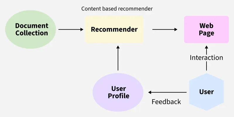
Recommender systems, particularly content-based filtering approaches, leverage cosine similarity to match user preference profiles against item feature vectors. In a movie recommendation engine, for instance, each film can be represented as a vector encoding genre weights, director style, keyword tags, and plot summary embeddings. A user profile vector is constructed by aggregating the vectors of items the user has positively interacted with. The system then computes cosine similarity between this user profile and all candidate items, surfacing those with the highest scores.
This approach extends naturally to collaborative filtering as well. Here, users and items occupy a shared latent space (often derived via matrix factorization), and cosine similarity between user vectors identifies neighborhoods of similar users whose preferences inform recommendations. The magnitude-invariant property is critical here: a power user who has rated 500 items and a casual user who has rated 20 should still be comparable based on the direction of their preference vectors, not the volume of their interactions.
Duplicate and Near-Duplicate Detection
Identifying duplicate or near-duplicate content is essential in data pipelines, plagiarism detection systems, and content moderation platforms. Cosine similarity provides an efficient mechanism for this task. Documents are vectorized, and pairwise cosine similarity scores above a defined threshold (commonly 0.85–0.95, depending on the strictness required) flag potential duplicates.
This technique handles paraphrased content effectively when combined with semantic embeddings rather than simple bag-of-words representations. However, practitioners should remain aware of a key limitation: cosine similarity can produce misleading results when documents contain antonyms or negations that reverse meaning without significantly altering the overall vector direction. Supplementing cosine similarity with additional semantic checks mitigates this risk.
Practical Considerations
When deploying cosine similarity at scale, keep these factors in mind:
- Sparse vs. dense representations: TF-IDF vectors are high-dimensional and sparse, making them efficient with sparse matrix operations. Dense embeddings (e.g., from BERT or sentence-transformers) are lower-dimensional but require approximate nearest neighbor libraries like FAISS or Annoy for performant retrieval.
- Threshold tuning: The similarity threshold for each application requires empirical calibration against labeled data. A threshold that works for duplicate detection will likely be too aggressive for semantic search.
- Preprocessing impact: Tokenization, stopword removal, and stemming decisions directly affect vector quality and, consequently, the reliability of cosine similarity scores.
Across all three domains, cosine similarity remains a robust, interpretable, and computationally efficient metric—one that translates naturally from linear algebra theory into high-impact production systems.
Best Practices and Key Takeaways
Cosine similarity remains one of the most widely adopted metrics in text analysis for good reason: it is computationally efficient, intuitive to interpret, and scales well across high-dimensional sparse vector spaces. However, as with any tool in the NLP practitioner’s arsenal, applying it effectively requires understanding both its strengths and its boundary conditions. Below, we distill the key takeaways and best practices to guide your implementation decisions.
Choose the Right Representation Before Measuring Similarity
The quality of your cosine similarity results depends entirely on the quality of your vector representations. When working with bag-of-words or TF-IDF representations, each unique word constitutes a dimension, and the frequency or weight of that word in a document defines the corresponding value. This transformation step is critical — poorly constructed vectors will yield misleading similarity scores regardless of how mathematically sound the metric is.
For modern applications, consider whether sparse representations (TF-IDF) or dense embeddings (Word2Vec, BERT, sentence-transformers) better suit your use case. Dense embeddings capture semantic relationships that sparse vectors miss, but they also change the interpretability profile of your similarity scores.
# Code snippet demonstrating cosine similarity computation using both
# TF-IDF vectors and dense sentence embeddings (e.g., via scikit-learn's
# cosine_similarity and sentence-transformers library)
import numpy as np
from sklearn.feature_extraction.text import TfidfVectorizer
from sklearn.metrics.pairwise import cosine_similarity
from sentence_transformers import SentenceTransformer

# Sample Data
corpus = [
    "The chef prepared a delicious meal.",
    "A cook is making some tasty food.",
    "The weather is quite rainy today."
]
query = ["The professional is cooking dinner."]

# --- Method 1: TF-IDF (Sparse / Keyword Matching) ---
tfidf_vectorizer = TfidfVectorizer()
tfidf_corpus = tfidf_vectorizer.fit_transform(corpus)
tfidf_query = tfidf_vectorizer.transform(query)

tfidf_sim = cosine_similarity(tfidf_query, tfidf_corpus).flatten()

# --- Method 2: Sentence-Transformers (Dense / Semantic Meaning) ---
# This uses a BERT-based model to understand that 'chef' and 'cook' are related
model = SentenceTransformer('all-MiniLM-L6-v2')
dense_corpus = model.encode(corpus)
dense_query = model.encode(query)

dense_sim = cosine_similarity(dense_query, dense_corpus).flatten()

# --- Display Comparison ---
print(f"Query: {query[0]}\n")
print(f"{'Document Content':<40} | {'TF-IDF':<10} | {'Dense':<10}")
print("-" * 65)
for i in range(len(corpus)):
    print(f"{corpus[i]:<40} | {tfidf_sim[i]:.4f}     | {dense_sim[i]:.4f}")

# Output:
"""
Query: The professional is cooking dinner.

Document Content                         | TF-IDF     | Dense
-----------------------------------------------------------------
The chef prepared a delicious meal.      | 0.2513     | 0.6795
A cook is making some tasty food.        | 0.2277     | 0.6177
The weather is quite rainy today.        | 0.4736     | 0.0349
"""
Understand the Magnitude-Independence Trade-Off
One of cosine similarity’s defining properties is its magnitude independence — it measures only the angle between two vectors, not their absolute sizes. This makes it particularly useful for comparing documents of vastly different lengths, since a 500-word article and a 5,000-word report can still register as highly similar if their term distributions align proportionally.
However, this same property introduces a well-documented deficiency. As research on the Vector Similarity Metric (VSM) highlights, cosine similarity yields identical values for vector pairs that differ dramatically in magnitude, so long as the angle between them remains constant. In practice, this means two documents could score a cosine similarity of 0.95 even when one contains term frequencies orders of magnitude larger than the other. For applications where volume or intensity of term usage matters — such as sentiment strength detection or frequency-based ranking — you should supplement cosine similarity with magnitude-aware metrics like Euclidean distance or the proposed VSM.
Guard Against Semantic Blind Spots
Cosine similarity operates on the geometric relationship between vectors and is inherently agnostic to semantics when used with traditional representations. It cannot distinguish antonyms from synonyms, nor can it account for negation. The sentence “This product is excellent” and “This product is not excellent” may produce deceptively high similarity scores in a bag-of-words model because they share most of their terms.
To mitigate this:
- Use contextual embeddings (BERT, RoBERTa) that encode negation and semantic nuance into the vector space.
- Preprocess deliberately — consider negation handling, stopword removal, and lemmatization as part of your pipeline.
- Validate with domain-specific test cases that include known edge cases like antonym pairs and negated phrases.
Practical Recommendations
- Normalize your vectors before computing cosine similarity when using custom implementations. Libraries like scikit-learn handle this internally, but manual implementations often omit this step.
- Benchmark against alternatives. For search engines and recommendation systems, evaluate cosine similarity alongside metrics such as Jaccard similarity, BM25, or learned similarity functions to determine which best fits your retrieval quality requirements.
- Profile performance at scale. Cosine similarity on sparse matrices is fast, but dense embedding comparisons across millions of documents benefit from approximate nearest neighbor libraries like FAISS.
- Interpret scores contextually. A cosine similarity of 0.8 means very different things depending on your vector space. Establish empirical thresholds through evaluation on labeled data rather than relying on arbitrary cutoffs.
Cosine similarity is not a universal solution, but it is an exceptionally reliable baseline. By pairing it with thoughtful preprocessing, appropriate vector representations, and an awareness of its geometric limitations, you can build text analysis pipelines that are both robust and interpretable. Treat it as a starting point — then validate, iterate, and augment as your application demands.
Frequently Asked Questions
Q: What is cosine similarity and how does it measure text similarity?
A: Cosine similarity measures the cosine of the angle between two vectors in a multi-dimensional space, producing a value between 0 and 1. When applied to text analysis, documents are converted into numerical vectors (e.g., using TF-IDF), and cosine similarity quantifies how similar their content is regardless of document length. A score of 1 indicates identical orientation (very similar text), while 0 indicates no similarity.
Q: Why is cosine similarity preferred over Euclidean distance for text analysis?
A: Cosine similarity is preferred because it measures the angle between vectors rather than their absolute distance, making it invariant to document length. Two documents discussing the same topic but of vastly different lengths will have similar cosine similarity scores, whereas Euclidean distance would penalize the length difference. This makes cosine similarity far more robust for comparing text in high-dimensional, sparse vector spaces.
Q: How do TF-IDF and the vector space model relate to cosine similarity?
A: TF-IDF (Term Frequency–Inverse Document Frequency) is a weighting scheme that transforms raw text into numerical vectors within a vector space model, where each dimension represents a unique term in the corpus. Cosine similarity is then applied to these TF-IDF vectors to compute document similarity. TF-IDF ensures that common words are down-weighted while distinctive terms are emphasized, leading to more meaningful similarity scores.
Q: How do you implement cosine similarity in Python for NLP tasks?
A: In Python, you can compute cosine similarity using scikit-learn’s TfidfVectorizer to create TF-IDF vectors and cosine_similarity from sklearn.metrics.pairwise to compare them. Alternatively, you can use NumPy to manually compute the dot product divided by the product of vector magnitudes. For deep learning-based text embeddings, libraries like sentence-transformers provide pre-trained models that generate dense vectors suitable for cosine similarity computation.
Q: What are common real-world applications of cosine similarity in NLP?
A: Cosine similarity is widely used in search engines to rank documents against user queries, in recommendation systems to suggest similar articles or products, and in plagiarism detection to flag duplicate content. It also powers semantic search with text embeddings, document clustering, chatbot intent matching, and duplicate question detection on platforms like Stack Overflow and Quora.